Theory of Thyroid Statistics - Z-story - DRAFT 1/02/2025

The null hypothesis is the starting point of statistical analysis. It states,

There is no effect - there is no problem - prove me wrong.

In order to diagnose the presence of disease in a patient, statistical evidence must be presented that "it is unlikely" that a healthy patient will present with the particular lab test. In this case, we reject the null hypothesis and accept the alternate hypothesis that there is sufficient statistical certainty that there is an effect, problem, or disease.

When the statistical certitude that the null hypothesis can be rejected reaches a certain threshold, then it is said that there is statistically significant evidence that the alternative hypothesis (that the patient is diseased) should be accepted. Typically, in medicine, there must be a statistical certitude of at least 95% that the null hypothesis can be rejected for the alternate hypothesis that the patient has an effect, problem, or disease to be accepted. Put another way, there is less than 5% certitude that the patient is "normal." This certitude is often expressed as "having statistical significance at p = 0.05").

Various statistical techniques can estimate the reference range (the 95% confidence interval). The most straightforward approach is to collect 1,000 apparently healthy individuals and run the lab test on them. Results are expected to vary according to random chance. If the 1,000 lab values are sorted from lowest to highest, and the 25 lowest and 25 highest values are discarded, then the range of the remaining values will represent the "middle" 95% of the sample. The lowest and highest remaining values represent an estimate of the reference range. This procedure only gives a statistical estimate based on a sample of 1,000 individuals. If the process were repeated with a new group of 1,000 apparently healthy individuals, then a similar but not the same reference range is expected. A less repeatable reference range would be obtained if a smaller sample size were used (e.g., 200 healthy individuals and "trim" off the highest 5 values and the lowest 5 values). A larger sample size would give more repeatable results. The method described here is non-parametric, which means that it does not depend on any assumption of special properties of the data, such as "normal distribution" (see below). In practice, labs may base their reference ranges on statistical techniques that assume the data follows a normal distribution; these reference ranges are only reliable if the statistical assumptions made are valid. Regardless of how the reference range is obtained, it is treated as a uniform (rectangular) distribution in which any lab test value within the reference range equally satisfies the null hypothesis, and any value outside the reference range equally rejects the null hypothesis, which leads to all-or-nothing decision making, as described below.

Boolean logic is a system of decision-making that is based on "true" and "false" with no intermediate "shades of gray." The conventional medical view taught and practiced by allopathic MDs uses Boolean logic to reason with test results. A given test result is classified as either "in the reference range," which means that it is FALSE that the patient has a problem, or "outside the reference range," which means that it is TRUE that the patient has a diagnosable problem. If the reference range is 0.50 to 4.50, for example, a patient with a test result of 0.51 is treated the same as a patient with a test result of 4.49 - i.e. is "within normal limits" and therefore has no diagnosis of disease. The patient is put into a "box" 4 units wide. Just a smidge to the left or right would cause the patient to fall out of the box and be classified as "abnormally low" or "abnormally high." This view may cause patients near the edges of the box who would benefit from treatment to be told that they are "normal" and to be denied treatment.

The distribution of many measured values subject to random independent variations tends to follow a "Gaussian," "normal," or "bell-shaped" distribution that approximates a binomial distribution. In particular, if the lab test results of many people are affected by random individual variation, then a graph of the values will be approximately normally distributed, and standard statistical techniques are applicable. In this view, the null hypothesis is most likely to be satisfied at the center of the "hump" of the bell curve and is progressively less likely to be satisfied as the patient's lab value moves left or right toward the "tails" of the bell curve.

This bell-shaped distribution assumption is not a perfect reflection of reality. However, it is a better approximation of reality than the uniform rectangular distribution implied by the conventional approach used by allopathic MDs as described above. As will be discussed below, fuzzy medical decision-making based on the assumption of a normal distribution of test results (e.g., statements like the patient's lab has a Z-score of -1, which means we are about 68% certain that the patient's lab value is abnormal) is expected to be more precise than Boolean medical decision-making using the "in the box/out of the box" approach of assuming a uniform rectangular distribution (which for that same patient we would say "the patient is normal)."

Any Gaussian distribution curve can be characterized by the population mean (μ) and the standard deviation (σ). The population mean is the value that represents the top of the hump of the bell curve; the standard deviation is a measure of "how wide" the bell curve is. Without delving into all the mathematics, it can be shown that there is a simple approximate relationship between the reference range described in the conventional medical view and the population mean and standard deviation:

Let L and U represent the lower and upper bounds of the 95% reference range obtained as above (when applied to data that follows an approximately normal distribution).

Then the population mean = μ = (L+U)/2, and the standard deviation = σ = (U-L)/2 .

It is convenient to convert (transform) a patient's lab values into Z-scores.

The following formula converts the measured lab value (denoted V) to its corresponding Z-score (denoted Z):

Z = 2 * (V - μ) / σ

These transformed values have the following convenient properties according to the 68-95 rule:

• Z = 0 means that the patient's lab value is in the middle of the reference range and is most likely normal (the patient is normal from an allopathic perspective);
• Z < -2 means that the patient's lab value is lower than the 95% reference range - reject the null hypothesis at a level of p=0.05 (we are more than 95% certain the patient has a diagnosable disorder from an allopathic perspective);
• Any Z value between -2 and +2 lies within the 95% reference range (within 2 standard deviations of the middle) - accept the null hypothesis at a level of p=0.05 (we are less than 95% certain the patient has a diagnosable disorder, so the patient is considered normal from an allopathic perspective);
• Z > +2 means that the patient's lab value is greater than the 95% reference range - reject the null hypothesis at a level of p=0.05 (we are more than 95% certain the patient has a diagnosable disorder from an allopathic perspective);
• Z-scores are real numbers with a continuum of values representing shades of gray (naturopathic and functional medical perspective)- not just true and false (allopathic medical perspective).

An advantage of Z-scores is that the reference range is always from -2 to +2, so it is easy to tell where a lab value lies relative to the reference range (low, normal, high). Even more powerful, since Z-scores are continuous, degrees of belief in the null hypothesis can be expressed by intermediate values. If we assume that the test data is approximately normally distributed (which follows from the Central Limit Theorem of statistics), then given the 95% upper and lower bounds of the test data (L and U) and the patient's test value (V), then we can calculate a Z value as follows. For example, consider the case of TSH (reference range = 0.45 to 4.5) and a measured lab value = 3.5, as follows:

Example:

L = 0.5, U = 4.5, and V = 3.5; then

Z = 2 * (V - ?) / ? = 2 * (3.5 - 2.5) / 2 = +1.0

I.e., the patient's lab value is 1 standard deviation higher than the mid-range.

Based on the 68-95 rule, we are 68% certain the null hypothesis can be rejected, which means we are 68% certain the patient has a problem that deserves intervention. Do we wait until we are more than 95% certain the patient has a problem, or do we begin mild interventions sooner rather than wait for the patient to cross the line into 95% certainty of abnormality? Where do we draw the line between intervention and watchful waiting?

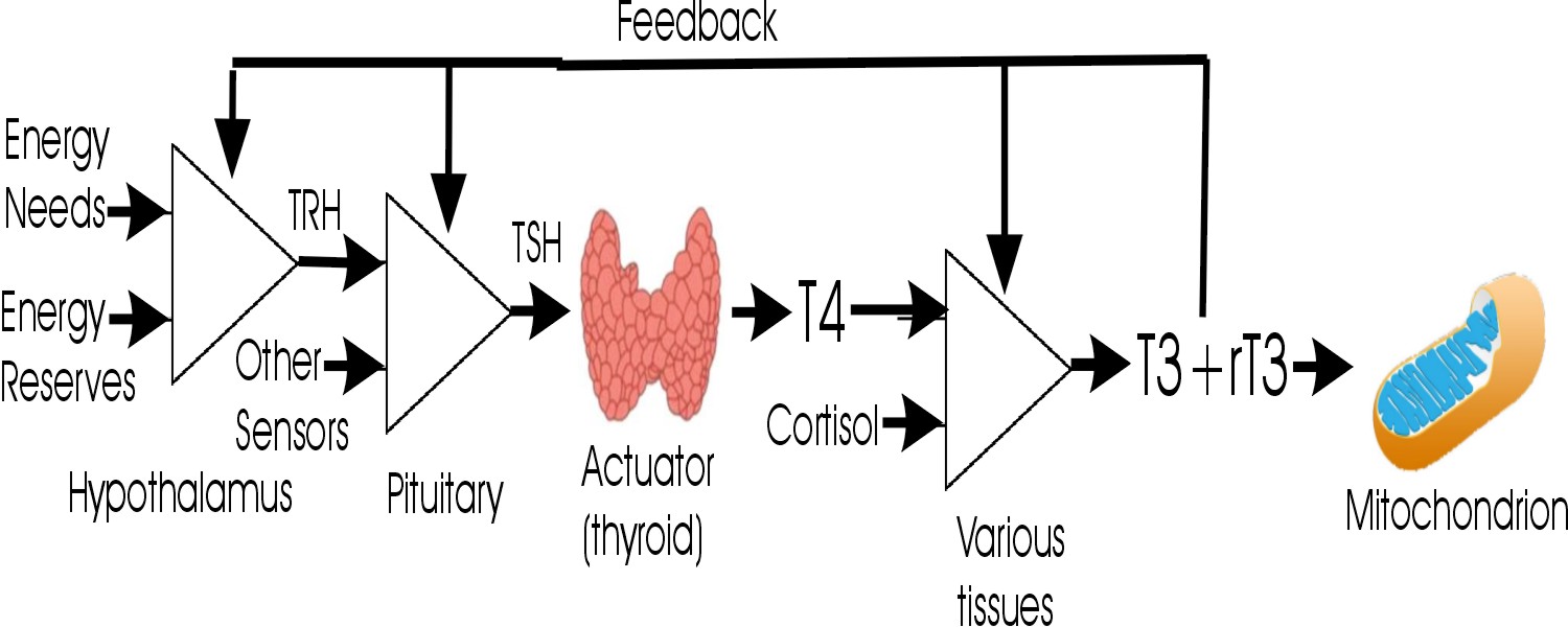
In the absence of any specific information to the contrary, we assume that the optimal value for a lab value is the center of the reference range, where Z = 0. In other words, the center of "normal" = "optimal." For example, in the thyroid system, a patient is in optimum balance when Z(TSH) = Z(T4) = Z(fT4) = Z(T3) = Z(fT3) = Z(rT3) = 0.

In the absence of any specific information to the contrary, we assume that for a process in which one precursor is converted through one or more steps to a product, if the conversion pathway proceeds at a normal rate, then the Z value of the precursor should be proportional to the Z value of the product. Note that if Z(precursor) > Z(product), it may imply either an abnormally active subsequent step is siphoning off the product or the conversion is impaired. For example, in the thyroid pathway, Z(T4) should equal Z(T3) and also equal Z(rT3) in the case of "normal rate of conversion."

In the absence of any specific information to the contrary, we assume that if a process in which a control substance causes the production of a product proceeds at a normal rate, the Z value of the control substance should be equal to the Z value of the product. For example, in the thyroid pathway, Z(TSH) should equal Z(T4).